Scaling search to terabytes on a budget

In this blog post, we indexed 23 TB of data and evaluated search performance and costs.

TLDR:

• Indexing costs $2 per ingested TB. Indexing throughput scales linearly with the number of indexers.
• Search costs $0.0002 per TB for a single full-text search or analytical query. Search latency behaves as $L = A/N + B$ where N is the number of searchers and $B\geq500ms$.
• Storage costs $0.3 per ingested TB with 1 day of retention (assuming the activation of inverted index, columnar, and row-oriented storage modes across all document fields).

At Quickwit, our mission is to engineer a cloud-native search engine. We focused on append-only data, and we strive to make it fast and efficient. Hence, our motto: "Search more with less".

But how does it work in practice? As of now, we haven't shared any official benchmark for our engine, and we receive a lot of questions from new users:

• How fast is Quickwit?
• Does it scale?
• Given my usage, how much will it cost me?
• How many GET/PUT requests to the object storage should be expected?

Many of these questions can be tricky to answer as their answers depend on:

• The dataset.
• The workload. In particular, are the queries traditional search queries, or are they analytical queries?
• Multi-tenancy specific configuration.
• QPS (Query Per Second).
• Etc.

Generally speaking, there is no straight answer, and the famous adage "No silver bullet" holds. Ultimately, it's all about tradeoffs, and the better you understand the engine, the easier you make the right choices. I spent hours and even days writing long, detailed explanations on Discord, private slacks, or other channels to share that knowledge with our community.

Through this post, my goal is to give you technical insights about the engine and demonstrate its performance on a relatively large dataset (~23TB). This knowledge will help you make the right choices to fit your unique requirements.

Before diving into the performance, let's start with a Quickwit 101, so you can understand the engine's inner workings.

Quickwit 101​

Decoupling Compute and Storage​

At the heart of Quickwit's architecture lies the principle of decoupling compute and storage¹. Our approach is very similar to (but predates) what Datadog did with Husky, and the goal is identic: cost-efficiency and scaling without cluster management nightmares.

This approach led us to separate completely the indexing (write path) and the search (read path). Both writers and readers share the same view of the world via a metastore. While indexers write to the storage and update the metastore, searchers read data from storage and the metastore.

In the current state of Quickwit, the metastore is traditionally backed by a PostgreSQL database. But Quickwit has a simpler implementation where the metastore is backed by a simple JSON file stored on the object storage; no need to rely on an external database for simple cases². That's the chosen setup for this blog post.

Indexing​

To feed Quickwit, you typically send JSON documents to the indexer's ingest API. The indexer then "indexes" them: it chops the stream of documents in short batches, and for each batch, it creates a piece of the index (concretely a file) called "split". The time interval at which we emit these splits can be configured (See commit_timeout_secs). These splits are then uploaded to S3.

Upon upload initiation, the indexer marks the split metadata within the metastore as Staged. Once the upload is finished, this state transitions to Published, indicating the split's availability for searching. The interval spanning a document's ingestion to its search readiness is called the "time to search", which roughly equals commit_timeout_secs + upload_time.

These steps are materialized by a processing pipeline, detailed further in this related post.

Unpacking the 'Split'​

To provide context for search queries, it's essential to grasp what a "split" contains as this is the unit of data of an index. It is an independent index with its schema, packed with data structures optimized for fast and effective search and analytics operations:

• Inverted index: Used for full-text search. For the curious keen to delve deeper, I can only encourage you to read fulmicoton's blog posts [1] and [2].
• Columnar storage: Used for sorting and analytics purposes.
• Row-oriented storage: Used for document retrieval by their ID.
• Hotcache: Think of it as an index's blueprint. Containing metadata from the previous data structures, it ensures searchers retrieve only essential data. The hotcache is the first piece of data retrieved by the searchers; it is generally kept in memory.

For illustration, let's take a real-world example of a split housing 10 million GitHub Archive events for which all data structures are enabled across all document fields.

The split size is roughly 15GB. Compared to the uncompressed size of the documents, it shows a compression ratio of almost 3. Note that optimizing this ratio is possible by enabling specific storages only on relevant fields.

Finally, the hotcache shows a nice property: it represents less than 0.1% of the split size, around 10MB, which means it could easily fit in RAM.

A word on merges​

You may wonder how Quickwit manages to generate 10 million-document splits while the indexer can commit every 10 seconds. The answer lies in Quickwit's merge pipeline, which takes care of merging a group of splits until it reaches a given number of documents³. This is useful for two main reasons:

• Performance Enhancement: You don't want to open many tiny splits on each search request. It also considerably reduces the amount of data our metastore has to handle. Thanks to merges, we end up having one row in PostgreSQL for every 10 million documents.
• Cost efficiency: You're happy to limit the number of GET requests on each search request.

Search​

On the read side, when a searcher receives a search request, it goes through these steps:

1. Metastore Retrieval: The searcher fetches the metastore.json file.
2. Split Listing: It lists relevant splits for the search request. This phase notably uses the search request's time range to eliminate splits that don't match the time range⁴.
3. Leaf Search Execution: For each split, a concurrent « leaf search » is performed. It includes:
   1. (IO) Retrieving the split's hotcache.
   2. (IO) Warmup phase: For each term, it fetches the posting list byte ranges and then the posting list itself. If necessary, it also fetches positions and columns required for the search⁵. For readability, the warmup phase is represented as a single fetch on the diagram below, but in reality, it can be multiple fetches.
   3. (CPU) Search phase: Runs the query on the split.
4. Result Aggregation: The leaf search results are merged.
5. Document Fetching: The searcher fetches the documents from related splits.
6. Result Return: The matching documents and/or aggregations are finally returned to the user.

This results in the following read path:

The Metastore​

Let's return to the shared view of indexers and searchers: the metastore. It stores the critical information about the index that we partly saw in the previous sections:

• Index configuration: document mapping, timestamp field, merge policy etc.
• Splits Metadata: If your dataset has a time field, Quickwit notably stores the min and max timestamp values for every split, enabling time-based filtering at search time.
• Checkpoints: For every datasource, a "source checkpoint" records up to which point documents have been processed. If you use Kafka as a datasource, the checkpoints contain each partition's start and end offsets indexed in Quickwit. That's what unlocks the exactly-once semantics.

The metastore can be powered by PostgreSQL or a single JSON file stored on the object storage. The latter is used for this blog post as it's the most straightforward setup. Here's a snapshot of the metastore's content:

{
    "index_uri": "s3://indexes/{my-index}",
    "index_config": {...},
    "splits": [
        {
            "split_id": "...",
            "num_docs": 10060714,
            "split_state": "Published",
            "time_range": {
                "start": 1691719200,
                "end": 1691936694
            },
            "split_footer": {
              "start": 1612940400,
              "end": 1616529599
            }
            ...
        }
    ],
    "checkpoints": {
      "a": "00000000000000000128",
      "b": "00000000000000060187",
      ...
    }
}

Did you notice the intriguing split_footer field? That's... the byte range of the hotcache!

Distributing Indexing and Searching​

Distributing indexing and search introduces some challenges:

• Cluster Formation: Quickwit uses an OSS implementation of Scuttlebutt called Chitchat to form clusters.
• Metastore Writes: On the write path, only one process should process the writes to the metastore file⁶. To this end, a single metastore role instance reads/writes the JSON file. Other cluster members send read/write gRPC requests to this instance.
• Indexing Task Allocation: One control plane role oversees indexing tasks distribution to individual indexers.
• Search Workload Distribution: This requires a map-reduce mechanism. The searcher receiving a search request assumes the "root" role, delegates leaf requests to "leaf nodes", then aggregates and returns the results.

Here's a visual representation of the write path:

Similarly, for the read path:

For a more comprehensive dive, explore our documentation.

Benchmark Setup​

Selecting an Adversarial Dataset​

Back in my high school years, I was deeply into fencing, competing at the national level. One lesson that stuck with me was the importance of a worthy adversary: a sparring partner, who pushes you beyond your comfort zone. For Quickwit, it's not that different. We are looking for a similar challenge in the form of a demanding dataset, and we found our match in the GitHub Archive.

Here’s why it's a good fit:

• Scale: With 23TB of data and 6 billion documents, you get a good sense of the scalability.
• Complexity: The JSON documents represent different kinds of events, all with different properties. As a result, the archive comprises thousands of fields, including lengthy text sections. This is perfect for stressing the used data structures on read and write.
• Track Record: The GitHub Archive has already been valuable for bug identification, most recently uncovering a bug in memory usage tracking.
• Relatability: Every developer can understand it and easily imagine fun queries to run against it.

Here's a glimpse of a typical document from this dataset:

{
  "id":"26163418660",
  "type":"IssuesEvent",
  "actor":{
    "id":121737278,
    "login":"LaymooDR",
    "display_login":"LaymooDR",
    "url":"https://api.github.com/users/LaymooDR",
    ...
  },
  "repo":{
    "id":383940088,
    "name":"ShadowMario/FNF-PsychEngine",
    ...
  },
  "payload":{
    "action":"opened",
    "issue":{
      "url":"https://api.github.com/repos/ShadowMario/FNF-PsychEngine/issues/11628",
      "id":1515231442,
      "title":"Chart Editor glitched out and overwrote a completed chart with a blank chart",
      "user":{
        "login":"LaymooDR",
        "avatar_url":"https://avatars.githubusercontent.com/u/121737278?v=4",
        ...
      },
      "state":"open",
      "body":"### Describe your bug here.\n\nJson was reloaded, but it never did anything. The chart was then saved, accidentally overwriting the chart, with no way to recover it.\n\n### Command Prompt/Terminal logs (if existing)\n\n_No response_\n\n### Are you modding a build from source or with Lua?\n\nLua\n\n### What is your build target?\n\nWindows\n\n### Did you edit anything in this build? If so, mention or summarize your changes.\n\nNo, nothing was edited.",
      "reactions":{
        "url":"https://api.github.com/repos/ShadowMario/FNF-PsychEngine/issues/11628/reactions",
        "total_count":0,
        "+1":0,
        "-1":0,
        ...
      }
    }
  },
  "created_at":"2023-01-01T00:00:00Z"
}

Crafting a comprehensive config​

To truly evaluate Quickwit’s capabilities, we want to use the main features. Our approach involves:

• Using the inverted index across all fields.
• Using the columnar storage (aka as fast field) for all fields, excluding the five fields with extensive text. Such columns will enable fast analytics queries on almost every field.
• Using the row storage (aka doc store) for all fields.

Such a configuration gives us a baseline that you should be able to beat in most cases. It will also highlight the engine's weak spots. Hopefully, after reading this, you will not experience nasty surprises! But if you stumble upon any, I'm keen to hear about your experience. Reach out to me on Twitter/X or Discord.

Below is an extract of the index configuration tailored for our dataset (full config):

version: 0.6
index_id: gh-archive
doc_mapping:
  field_mappings:
      - name: payload
        type: object
        field_mappings:
        - name: title
          type: text
        - name: body
          type: text
      - name: issue
        type: object
        field_mappings:
        - name: title
          type: text
        - name: body
          type: text
    - name: created_at
      type: datetime
      fast: true
      input_formats:
      - rfc3339
  timestamp_field: created_at
  mode: dynamic

You might wonder, "What happened to the thousands of fields?" The trick is in the dynamic mode. By default, it integrates the inverted index, columnar storage, and doc store for fields not explicitly declared in the doc mapping.

Deployment & Infrastructure​

1. We deployed Quickwit on EKS with our helm chart, chart values are available here.
2. AWS's S3 takes charge of storing both the splits and the JSON metastore file.
3. We've allocated up to 24 indexers c5.xlarge - each with 4CPUs, 8GB RAM, and priced at $0.1540/h.
4. And up to 32 searchers c5n.2xlarge, each with 8CPU 21GB RAM and a rate of $0.4320/h.
5. Indexing the dataset is done with an experimental HTTP datasource⁷, which fetches data directly from https://www.gharchive.org/. Each indexer is assigned 1/nth of the dataset.
6. A Prometheus instance to collect metrics.
7. A Grafana instance to show you some beautiful charts.

With the stage set, let’s dive into indexing performance.

Benchmark results​

Indexing performance​

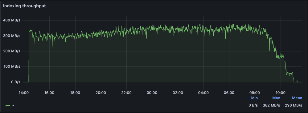Figure: Indexing throughtput with 12 indexers

I tested different numbers of indexers, from 1 to 24, each responsible for indexing 1/nth of the dataset. Knowing the GitHub Archive URLs follow the schema https://data.gharchive.org/20{15..24}-{01..13}-{01..32}-{0..24}.json.gz, each indexer took care of 24/nth URLs per day.

Post-indexing, our index has the following characteristics:

• Indexed Documents: 6.1 billion (spanning 2015 to 2023).
• Index Size: 8.4TB (yielding a compression ratio of 2.75).
• Number of Splits: 715.
• Documents per Split: An average of 8.5 million.
• Average Throughput: For an active indexer, it was 27MB/s. Note: An indexer becomes inactive once it completes indexing its dataset portion.

Here are the results in detail. Note that while 27MB/s is already relatively fast, this is on the low end of what we typically observe (20MB/s - 50MB/s).

Key Takeaways:

• Scalability: Throughput scaled linearly for active indexers. No noticeable metastore overhead was observed, though there were minor latency spikes in metastore gRPC calls. Their impact on indexing was minimal. The primary variation among indexers resulted from the dataset's inherent variations, leading to unequal data ingestion across indexers. In a 24-indexer setup, the initial indexer ended indexing in 7 hours, while the final one took 9 hours.
• Resource Utilization: Each indexer nearly maxed out the capabilities of a c5.xlarge, leaving limited scope for further optimization. There's potential to experiment with Graviton instances for comparison. Suggestions for other possible improvements are welcomed!
• Split Generation & Storage Requests: In this setup, Quickwit creates a split roughly every minute, triggering one PUT request for each new split and three multipart PUTs for merged splits⁸. The dataset's indexing required around 10k PUT requests.

Indexing costs​

Indexing costs mainly come from instance costs. S3 PUT request costs ($0.005 per 1000 requests) are comparatively negligible. The total cost of indexing is thus for 23 TB:

Total cost = $0.1540/h * 23 TB / 27 MB/s / 3600s/h = $36.4
Cost per TB = $1.58/TB

With 24 indexers and an average throughput of 22MB/s:

Total cost = $0.1540/h * 23 TB / 22 MB/s / 3600s/h = $44.7
Cost per TB = $1.94/TB

Search performance​

The main objectives of this benchmark are:

• Evaluating the performance across 4 typical queries, integrating both full-text search and analytics (aggregations), with searcher counts ranging from 1 to 32.
• Understanding the various cache mechanisms available in-depth.
• Estimating associated costs.

While we want to go into the details of each query, the benchmark doesn't aim to be exhaustive. A more detailed set of queries, coupled with comparisons to other search engines, will be featured in an upcoming blog post.

Four Queries Benchmarked​

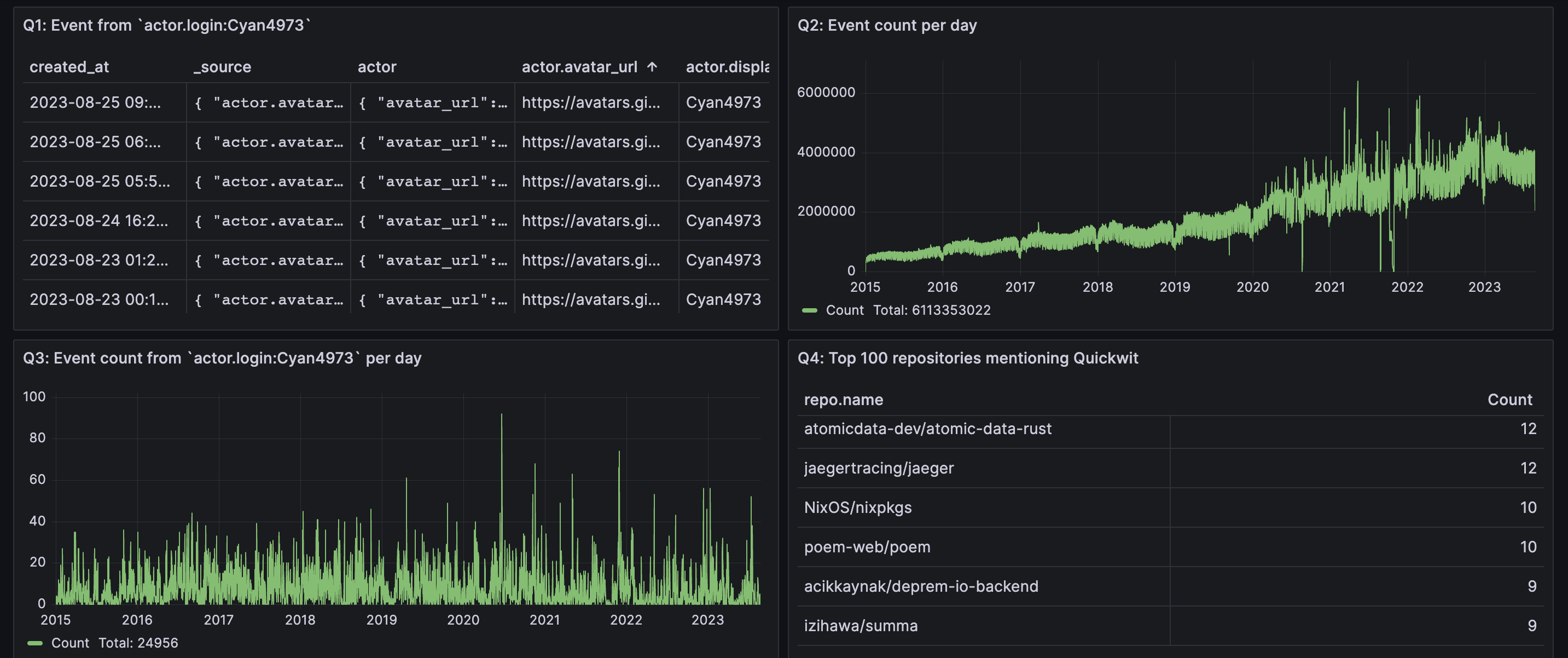Figure: Grafana dashboard showing the results of the four queries

• Q1: A term query on one field: actor.login:Cyan4973. Cyan4973 is the GitHub handle of Yann Collet, the brains behind LZ4 and ZSTD. This query hits 22k docs, but only the top 10 documents is returned.
• Q2: A date histogram query that counts events by day. This query scans all the dataset.
• Q3: A date histogram query focused on Cyan4973 events, aggregating over 22k documents.
• Q4: A term aggregation combined with filters on three text fields. The goal here is to identify the top 100 repositories by star count that mention "Quickwit" in event descriptions, comments, or issues.

Appendix provides the JSON body of each query

Different shades of cache​

Quickwit offers several caching mechanisms to boost search request speeds:

1. Split Footer Cache or Hotcache. As you already guessed, this cache bypasses the need to fetch the hotcache for every split. Keeping the hotcache in memory is generally recommended, as a search will fetch it for each query. You can configure it via split_footer_cache_capacity; its default value is 500M.
2. Fast Field Cache. This cache stores the columns necessary for the search query for each split. If your query sorts fields or performs an aggregation, Quickwit retrieves the columns of those required fields. For standard queries sorted by timestamp, it's wise to allocate this cache according to the size of the timestamp column. You can configure it via fast_field_cache_capacity; its default value is 1G.
3. The partial request cache. It caches the search query results for each split; it's useful mainly for dashboards, and we won't use this cache in the benchmark.

Results without cache​

We immediately notice that, while the 90th percentile latency is inversely proportional to the number of searchers at the beginning, it rapidly tends to a plateau between 1.4s to 2.6 second (Q4). This plateau is attributed to S3 latency. As we increase the number of searchers, we end up being IO-bound, each searcher is just waiting for the data coming from the object storage.

Detailing the IO operations performed by the searchers reveals:

• For every query, the hotcache for all splits is fetched, representing 715 GET requests and a data download of 6.45GB.
• Both Q1 and Q4 pull the posting lists for the term Cyan4973, leading to 1340 GET requests and a 10MB data download.
• Q2 and Q3 access the timestamp fast field, translating to 715 GET requests and 13.4GB of data.
• Q4 retrieves the repo.name column (32.7GB) and the posting list for the term quickwit for three fields, amounting to a few tens of MB.

To verify these numbers, I send the Quickwit's traces in our production Quickwit cluster that serves as a Jaeger backend, a bit of dogfooding is always nice.

For each query, I performed a single run and manually gathered the metrics into this table:

From the data, we can note that:

• Only Q2 is CPU-intensive. However, even in Q2's case, most of the processing time is sunk into IO.
• There's considerable variation per split. This can be explained by the variations between split as well as S3 latency and throughput variations.

Of course, we can complain of S3 latency, but... still, it's worth noting its impressive throughput. For instance, parallelized GET queries can achieve a throughput of 1.6GB/s with just a single instance (as shown by Q1's 6.45GB download in 4 seconds).

Let's now explore how enabling the hotcache, the most logical cache to turn on, can improve performance.

Results with hotcache for Q1​

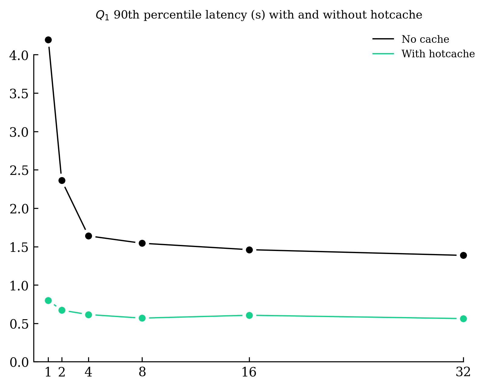
Caching all the hotcache, which demands 6.45GB, reveals significant improvements:

• Q1's 90th latency is now sub-second with 800ms with a single searcher.
• Across all queries, we witness an initial reduction of 2-4 seconds with one searcher. Then the reduction decreases gradually and tends to 300-800ms as we increase the number of searchers, which is expected as it mirrors the time taken to retrieve the hotcache.

Given the tiny footprint of the hotcache (less than 0.1% of the split), it's reasonable and advisable to size the memory of the searchers accordingly.

Remarkably, a single searcher with hotcache in cache can respond to a basic search query on 23TB under a second.

Results with hotcache and fast field cache for Q3​

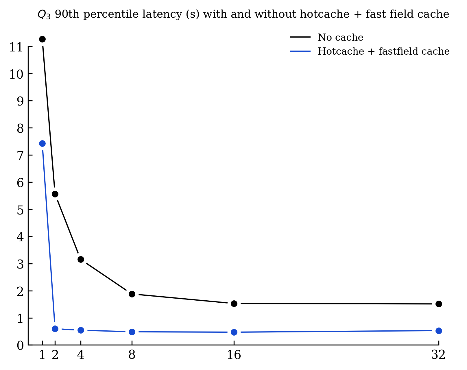
Executing Q3 demands retrieval of the hotcache, timestamp field, and posting lists. With two or more searchers, we can cache both the hotcache and fast field, leaving just the posting list retrieval. The anticipated outcome should mirror Q1 with hotcache, minus the document fetching duration (~100-200ms). This is validated by the observed latency: roughly 480ms, which is slightly quicker than Q1's 600ms.

Search costs​

Estimating search costs is a bit more tricky than indexing costs due to:

1. The GET request costs are no longer negligible. We have thousands of them for a single query.
2. The compute cost is harder to measure as the search latency does not reflect directly the CPU time.

To simplify the estimation, we can work on two types of queries to give a rough idea of the costs:

• Simple search queries (e.g., Q1 or Q3) where IO is the bottleneck. It takes less than 1 second of CPU to run them on 23TB.
• Analytical queries (e.g., Q2) are more CPU-intensive. Q2 takes around 30 seconds of CPU to run on 23TB.

Based on the number of GET requests, and assuming the hotcache is retained, their counts for each query type can be approximated as:

• Simple search queries: around 2000 GET requests for 23TB.
• Analytical queries: Roughly 3000 GET requests for the same data volume.

From here, we can deduce the costs for each query variety:

Wrapping up​

More than a benchmark, I hope this blog post gave you a better understanding of Quickwit's inner workings and how to use it efficiently.

We've got some exciting things coming in the following months that will open new use cases, and you may be very interested in them:

• Quickwit on AWS Lambda: As you probably guessed, Quickwit is well-suited for serverless use cases. Some users have already tested Quickwit on Lambdas and reported excellent results. We will make it easier to deploy Quickwit on lambdas and share a blog post about it.
• Local Disk Split Caching: As you noticed, Quickwit can fire a lot of requests to the object storage. When dealing with high QPS, the cost of GET requests quickly adds up when using object storage solutions like AWS S3. By caching splits, Quickwit will read bytes from the local disk instead of the object storage. This will significantly reduce the number of GET requests and the associated costs.

Stay tuned!

Appendix​

Q1 - Simple text search query​

{
  "query": "actor.login:Cyan4973"
}

Q2 - Count events per day​

{
    "query": "*",
    "max_hits": 0,
    "aggs": {
        "events": {
            "date_histogram": {
                "field": "created_at",
                "fixed_interval": "1d"
            }
        }
    }
}

Q3 - Top 100 repositories by number of stars​

{
  "query": "type:WatchEvent",
  "max_hits": 0,
  "aggs": {
    "top_repositories": {
      "terms": {
        "size": 100,
        "field": "repo.name",
        "order": { "_count": "desc" }
      }
    }
  }
}

Q4 - Top 100 repositories by number of stars mentioning Quickwit in events description, in comments, or issues.​

{
  "query": "(payload.description:quickwit OR payload.comment.body:quickwit OR payload.issue.body:quickwit)",
  "max_hits": 0,
  "aggs": {
    "top_repositories": {
      "terms": {
        "size": 100,
        "field": "repo.name",
        "order": { "_count": "desc" }
      }
    }
  }
}