In this blog post, we discuss the implementation of an indexable bitset in tantivy.

Picking the right building blocks​

Modern software engineering is about picking the right building blocks (libraries, data structures, databases, frameworks, or APIs) and interconnecting them. Many of us deplore this situation. They are nostalgic for the days when software was lean, and every codebase was its own little island with its own beautiful culture and idioms.

I personally think this change is for the best. Software engineering has matured, and our productivity has considerably increased as a result. One thing that irks me, however, is how branding is influencing our technological choices. If our only agency is choosing the right tool for the job, let's be smart and professional about it.

This blog post could have been a very short blog post: "We use Roaring bitmap because it is blazing fast"... But I suspect we are all very tired of those lazy shortcuts and all crave a proper long technical discussion.

Instead, in this blog post, I will explain our thought process in detail:

• What our problem was,
• Why we ended up picking up Roaring Bitmap,
• Why we tweaked it a bit,
• Where we think we could improve our current solution.

Why do search engines need a columnar format?​

Search engines are not just about search. Products like Quickwit or Elasticsearch are also great for interactive analytics. Let's have a look at the following dashboard backed by Quickwit thanks to our new Grafana plugins:

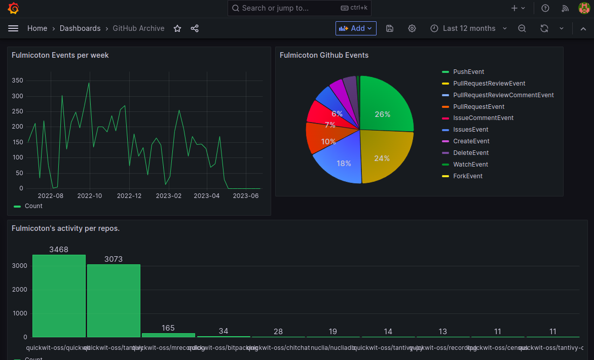
To compute the data displayed here, Quickwit wields together an inverted index and a columnar storage. (yes, Quickwit is ambidextrous)

Let's consider, for instance, the timeline graph on the top left. It shows my activity on GitHub using the GitHub archive dataset.

• The inverted index will give us an iterator over all of the events I am the author of.
• The columnar will provide a column of timestamps.

In pseudo-code, this computation will then look like this:

let mut date_histogram = DateHistogram::new();
let time_column = columnar.column("time");
for doc_id in inverted_index.search("author.id:fulmicoton") {
    let timestamp = time_column.get(doc);
    date_histogram.record(timestamp);
}
return date_histogram;

The time_column encodes a mapping from doc_id (a 32-bit unsigned integer) to timestamps.

In tantivy, this columnar format is called fast fields (Yes, I agree this is a terrible name). In Lucene, it is called DocValues (I will let you appreciate this one).

Until recently, tantivy's columnar format was very limited. In particular, we did not support sparse columns: fast fields were required to have values in all documents. We also required all fast fields to be explicitly declared in the schema.

To make Quickwit truly schemaless and offer a proper alternative to Elasticsearch for analytics, we had to make our columnar format more flexible. Here is how it works today.

Required, Optional, Multivalued cardinality

The columnar is just a dictionary of named columns. A Column<T> object carries:

• a dense column of values (ColumnValues<T>)
• an index that maps each doc_id to the right range of value in the column values (ColumnIndex)

The ColumnIndex is an enum, as it is encoded differently depending on the cardinality of the column:

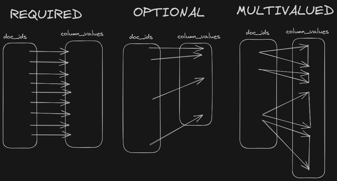
• Required: Every document has exactly one value. The mapping from doc_id to value_id is simply the identity function, and nothing needs to be stored.

• Optional: Every document has at most one value. As we will see, this index is equivalent to storing the set of documents having a value. This is precisely the optional index that I want to discuss.

• Multivalued: If a document can have any number of values. We simply encode a dense column with the start_row_ids of each document. The range is then given by start_row_ids.get(doc_id)..start_row_ids.get(doc_id + 1). We have specific codecs to efficiently compress the start_row_ids while allowing random access. But this is not the subject of this blog post.

We have finally reached the core of this blog post: Let's talk about how we encode the optional column index!

rank(..) and select(..)

As we have seen, an optional column index stores the set of documents holding a value.

We need two operations on this set, called rank (well, in our case rank_if_exists) and select. Don't blame me for the names this time. This is how these operations are called in the literature.

Let's have a look at a simple example first to get a proper intuition of what these two operations are about:

Here we are looking at a bitset containing the elements {2, 4, 6}. If we consider the list of sorted elements [2, 4, 6].

• 2 is at position 0. Therefore, rank_if_exists(2) = Some(0),
• 4 is at position 1. Therefore, rank_if_exists(4) = Some(1),
• 6 is at position 2. Therefore, rank_if_exists(5) = Some(2).

Simple, isn't it? select is then the inverse operation.

rank_if_exists​

rank_if_exists is used to access the value associated to a doc_id. It is typically called once for every document matching the query. Once we have the rank, it can be used to look up into a dense vector of values. The rust implementation of the function that fetches a value looks like this:

/// Returns the value associated with a given doc,
/// or None if there aren't any.
fn get_value<T>(column: &Column<T>, doc_id: u32) -> Option<T> {
    let value_id = column.column_index.rank_if_exists(doc_id)?;
    // column value here is a dense vector.
    Some(column.column_value[value_id])
}

Of course, as we search, we will call rank_if_exists with increasing values of doc_id. It is therefore tempting to rely on this access pattern and use a set representation that performs rank by skipping and scanning. That's how a column format like Parquet does it.

Lucene itself chose in LUCENE-7077 to lean toward an iterator interface for its DocValues. This was a bit of a controversial change at the time. Let's spell out the trade-off is:

• A sequential codec usually compresses better.
• A sequential codec might be less CPU efficient.

Some efforts like LUCENE-8585 alleviate the performance impact of scanning through doc values.

We made the other choice in tantivy. Our rank API allows for random access. Wherever it does not hurt compression too much, we want our indexable set to allow for a O(1) random access rank.

select​

Given a value_id, select answers the question, "To which document does this value_id belong?".

We have rank(select(value_id)) == value_id.

In Quickwit, we use this operation in range queries. You can read a little bit more about this in a previous blog post.

Contrary to rank, we tend to call select in batches. These batches are by nature less selective, so we do rely on a stateful iterator here. Fast random access is not necessary here.

Roaring bitmap with a minor twist

We want our bitset to be as small as possible and still offer fast rank operation and select operation. Ideally, we want the rank to offer fast random access.

Like Lucene, our compressed index is based on Roaring bitmaps, except our solution has a minor twist to accelerate rank operations.

The idea of roaring bitmaps is to partition our doc_id space in blocks of $2^{16}$ documents. For each block, depending on the number of documents we have, we use a dense or a sparse codec.

Dense blocks​

In roaring bitmap, a dense block is a bitset of 2^16 bits. Every single document, regardless of whether it is part of the set or not, takes exactly 1 bit.

In our codec, we added extra data to improve the performance of rank operations.

We split the block into 1024 mini-blocks of 64 elements each. Each mini-block then consists in:

• the rank (relative to the block) at the beginning of the mini-block: 16 bits,
• a bitset: 64 bits.

Each mini-block stores 64 documents and takes 80 bits. That's 1.25 bits per document.

rank​

rank is where our extra 0.25 bits come handy. Here is what the implementation of rank_if_exists looks like:

fn rank_u64(bitvec: u64, doc: u16) -> u16 {
    let mask = (1u64 << doc) - 1;
    let masked_bitvec = bitvec & mask;
    masked_bitvec.count_ones() as u16
}

pub struct DenseBlock<'a>(&'a [u8]);

struct DenseMiniBlock {
    bitvec: u64,
    rank: u16,
}

impl DenseBlock {
    /// `rank_if_exists` function running in O(1).
    fn rank_if_exists(&self, doc: u16) -> Option<u16> {
        let block_pos = doc / 64;
        let pos_in_block_bit_vec = doc % 64;
        let index_block = self.mini_block(block_pos);
        let ones_in_block = rank_u64(index_block.bitvec, pos_in_block_bit_vec);
        let rank = index_block.rank + ones_in_block;
        // This is branchless.
        if get_bit_at(index_block.bitvec, pos_in_block_bit_vec) {
            Some(rank)
        } else {
            None
        }
    }

    fn mini_block(&self, mini_block_id: u16) -> DenseMiniBlock {
        // ...
    }
}

If the data is in my L1 cache, on dense parts, the overall codec rank_if_exists implementation runs in 5ns on my laptop.

select​

Select is trickier. We do a linear search through the mini-blocks to find the block containing our target document. Once it is identified, we identify the exact document by popping bits from our 64-bits bitset.

fn select_u64(mut bitvec: u64, rank: u16) -> u16 {
    for _ in 0..rank {
        bitvec &= bitvec - 1;
    }
    bitvec.trailing_zeros() as u16
}

impl DenseBlock {
    fn select(&self, rank: u16) -> u16 {
        let block_id = self.find_miniblock_containing_rank(rank).unwrap();
        let index_block = self.mini_block(block_id).unwrap();
        let in_block_rank = rank - index_block.rank;
        block_id * 64 + select_u64(index_block.bitvec, in_block_rank)
    }

    fn find_miniblock_containing_rank(&self, rank: u16) -> Option<u16> {
        // just scans through the mini-blocks.
    }
}

In practice, a stateful SelectCursor object makes sure that we do not rerun over and over this linear search from the start. You can have a look at the implementation here.

Sparse block​

Following roaring bitmaps, our sparse blocks just store the 16 lower bits of our docs one after the other. How can we implement rank and select efficiently here?

rank​

We simply run a binary search. This isn't great, is it? Well, there is definitely a lot of room for improvement, and we might explore alternatives in the future. A good paper on the subject is Array layout for comparison based-search.

Thankfully, as we will see in the next section, there are at most 5,120 elements in sparse blocks. The loop body will be entered at most 13 times. Also, by nature, sparse blocks are less likely to show up in heavy queries.

impl<'a> SparseBlock<'a> {
    fn rank_if_exists(&self, el: u16) -> Option<u16> {
        self.binary_search(el)
    }

    fn binary_search(&self, target: u16) -> Option<u16> {
        let data = &self.0;
        let mut size = self.num_vals();
        let mut left = 0;
        let mut right = size;
        while left < right {
            let mid = left + size / 2;
            let mid_val = self.value_at_idx(data, mid);
            if target > mid_val {
                left = mid + 1;
            } else if target < mid_val {
                right = mid;
            } else {
                return Some(mid);
            }

            size = right - left;
        }
        None
    }
}

select​

Select is dead simple. We just have to perform a memory lookup. We can't do much faster, can we?

impl<'a> SparseBlock<'a> {
    fn select(&self, rank: u16) -> u16 {
        let offset = rank as usize * 2;
        u16::from_le_bytes(self.0[offset..offset + 2].try_into().unwrap())
    }
}

The cut-off​

We have seen that the dense bitset takes 1.25 bits per document in our segment, while the sparse codec takes 16 bits per element in the set. Obviously, we want to pick the dense codec for blocks with a lot of documents and the sparse codec for blocks with few documents (duh!).

Regardless of the number of elements in the set, a dense block always takes 10,240 bytes. On the other hand, a sparse block takes 2 bytes per doc in the block. The decision threshold, therefore, happens when we have less than 10,240 / 2 = 5,120 documents in the block.

Blocks metadata

We have discussed how we represent our blocks. We also need to talk a little about the metadata of that list of blocks.

It might seem like a trifle, but some datasets may present a very high number (hundreds, thousands!) of very sparse columns. For this reason, we need to make sure these super sparse columns only take a few bytes.

Today, we store the overall number of rows in the entire file as a VInt at the beginning of each column. This is a bit silly, as it is the same value for every column. I will ignore it in the computation below, but I had to confess this engineering sin.

We then store the sparse lists of non-empty blocks. For each block, we store

• the block_id (2 bytes)
• the number of elements in the block (2 bytes).

As we open a column, we read all of this metadata and expand it into a dense vector to allow for random access. We can afford this: there are at most a few hundred blocks per split.

A set with a single document in a 10 million split will therefore take 4 bytes of metadata, and 2 bytes for the actual document's lower bits. Overall, the smallest possible optional index will take 6 bytes.

For a dense set, on the other hand, our metadata will be negligible, and our column will take 1.25 bits per document in our segment. For an optional column in a split of 10 million documents, this is 1.5MB.

Are we compact?​

I avoided the use of the word compact so far as it has a very specific meaning in computer science. A compact data structure is smaller than some multiple of a theoretical minimum.

It happens that, no, our data structure is not really compact.

Now what does the theory tell us?

If we build a subset of $[\![0, M[\![$, by considering each element one by one and picking them with a probability $p$, Shanon's source coding theorem tells us we cannot do better (in average) than $M p log_2(p)$ bits to encode our set. This is also ${log_2}(p)$ per document in the set, depending on how you prefer to see it.

We can now plot the number of bits taken per document in the set for different values of $p$. Note we used here a log-scale for the X-axis.

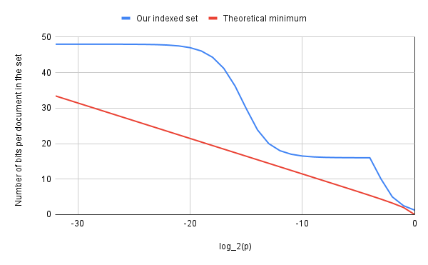
The graph shows two interesting spots, showing a lot of headroom. Around $p=1/2^{18}$, we are a bit larger than twice the theoretical minimum. In that range, most blocks will have one, two, or three elements. The culprit is our poorly compressed metadata.

The second spot is at around $P=1/13$, where we reach 3 times the theoretical minimum. Here we are at the limit between the dense and the sparse space. This is an interesting region because these are large columns. We might want to improve our compression here.

On the sparse side, this is also precisely the range where our rank performance also shows the largest performance headroom for the rank function.

Our codec does not qualify as "compact". It is, however, important to notice that roaring bitmaps have an edge over theory. In practice, documents are not independent. In a log dataset, for instance, documents are often sorted by time. A rare large request could generate a large trace presenting many spans with a given column. Roaring bitmaps are able to adapt to such changes of regime and hence break the floor of the theoretical minimum.

In conclusion​

To handle columns with an optional cardinality, we needed a way of encoding an indexable set. The set had to be reasonably well compressed and have a way to perform fast rank and select operations. Fast random access for rank operations was especially desirable.

We ended up copying Roaring bitmap and just augmented it to allow for fast rank operations in dense blocks. Thanks to this extra information, rank operation now takes a few nanoseconds, and our dense blocks are only 25% larger.

The theory also helped us identify significant headroom on compression and rank performance for sets with a density of around 1/13.

We haven't discussed other solutions like Partitioned Elias-Fano indexes or Tree-Encoded Bitmaps.

We simply did not investigate them. There are no efficient off-the-shelf implementations of these solutions, so we had to implement one. Roaring bitmap has the merit of being incredibly simple to implement and optimize.

Interestingly, if you skim papers about similar data structures, you may notice that they sometimes mention as "an exercise to the reader" the possibility to add extra data to get O(1) rank complexity... which is exactly what we did here!