Quickwit 101 - Architecture of a distributed search engine on object storage
In this blog post, we dive into Quickwit architecture and its key components. This blog post pairs best with Quickwit's benchmark on a 23TB dataset.

The inspiration behind Quickwit's logo stems from Paul's idea that software and kinetic art share an interesting characteristic. If you look at the beautiful work of Theo Jansen, you will see mesmerizing wind-powered sculptures walking on the beach, sufficiently complex to be unable to understand how it works. That feeling of intrigue is also akin to using software. Looking at large codebases, it seems a bit magical how such complex constructions can work... yet, more often than not, they do.
But we are engineers! We are not satisfied with magic, we want to understand how things work and don't make a decision based on the beauty of a software... (do we?). It is indeed critical to understand the inner working of an engine if we don't want it to blow up in our face and sleep well at night (I made that kind of mistakes too many times...). There is no need to cover all the details, a good mental model of the system is what we should target to understand its limits and how to use it efficiently.
And that's the blog post aim: diving into Quickwit architecture and its key components so you can build a concise and accurate mental model of the system. Time to dive in!
Decoupling Compute and Storage
At the heart of Quickwit's architecture lies the principle of decoupling compute and storage1. Our approach is very similar to (but predates) what Datadog did with Husky, and the goal is identic: cost-efficiency and scaling without cluster management nightmares.
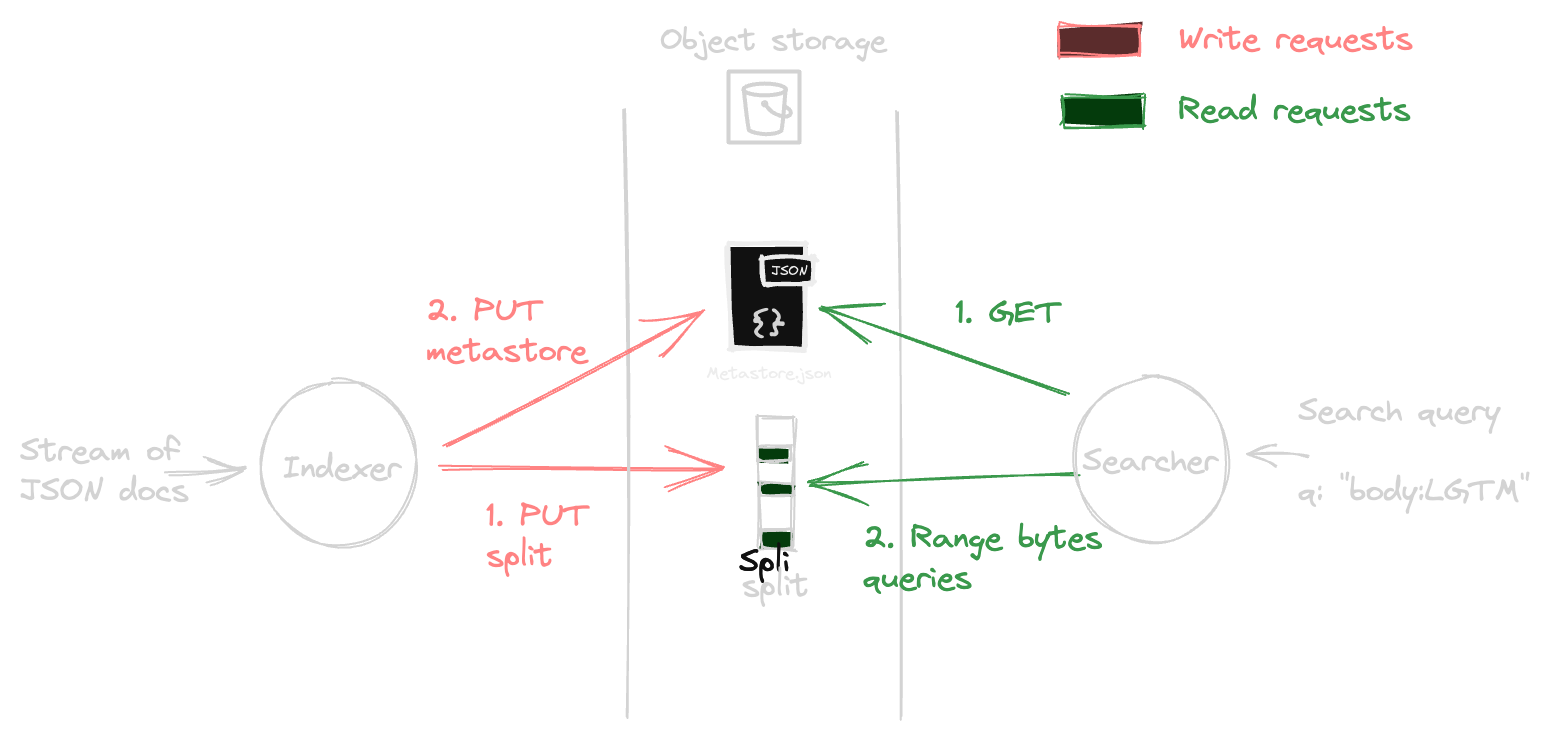
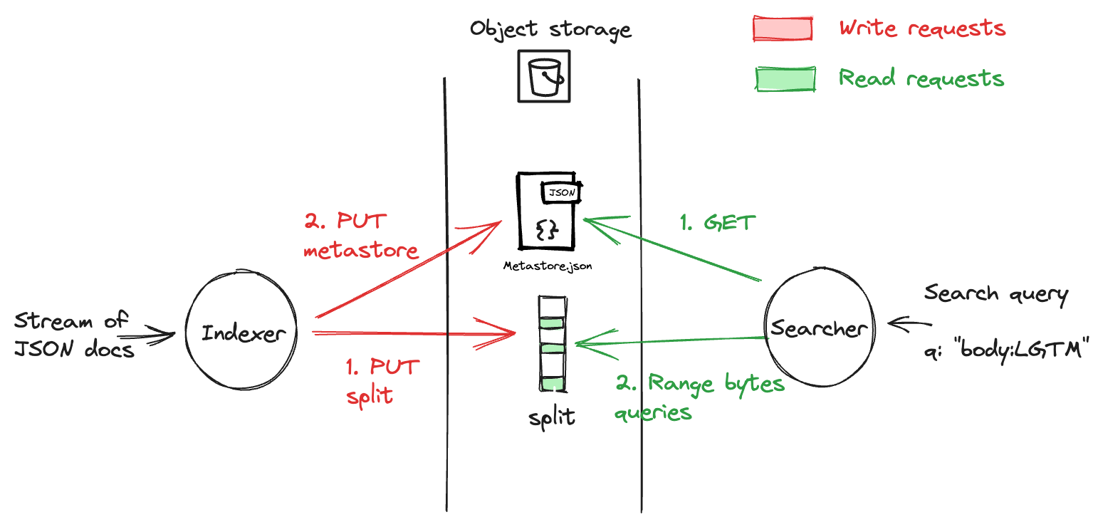
This approach led us to separate completely the indexing (write path) and the search (read path). Both writers and readers share the same view of the world via a metastore. While indexers write to the storage and update the metastore, searchers read data from storage and the metastore.
In the current state of Quickwit, the metastore is traditionally backed by a PostgreSQL database. But Quickwit has a simpler implementation where the metastore is backed by a simple JSON file stored on the object storage; no need to rely on an external database for simple cases2. That's the chosen setup for this blog post.
Indexing
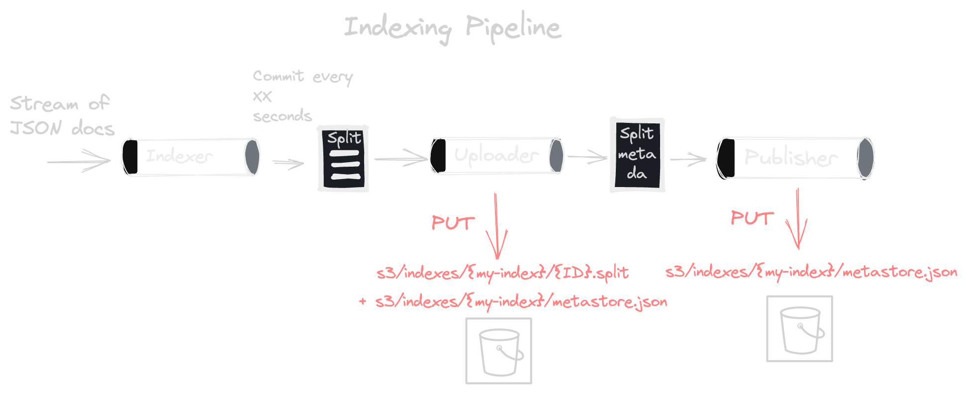
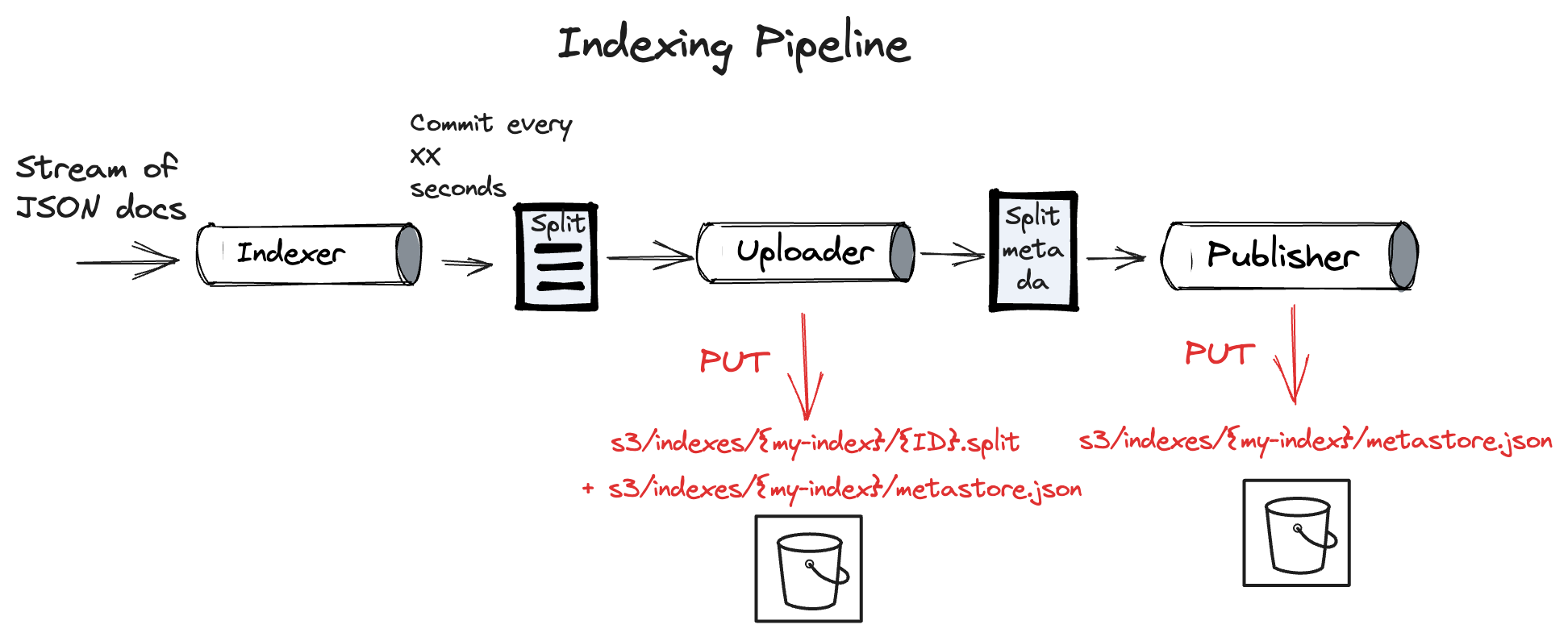
To feed Quickwit, you typically send JSON documents to the indexer's ingest API. The indexer then "indexes" them: it chops the stream of documents in short batches, and for each batch, it creates a piece of the index (concretely a file) called "split". The time interval at which we emit these splits can be configured (See commit_timeout_secs). These splits are then uploaded to S3.
Upon upload initiation, the indexer marks the split metadata within the metastore as Staged. Once the upload is finished, this state transitions to Published, indicating the split's availability for searching. The interval spanning a document's ingestion to its search readiness is called the "time to search", which roughly equals commit_timeout_secs + upload_time.
These steps are materialized by a processing pipeline, detailed further in this related post.
Unpacking the 'Split'
To provide context for search queries, it's essential to grasp what a "split" contains as this is the unit of data of an index. It is an independent index with its schema, packed with data structures optimized for fast and effective search and analytics operations:
- Inverted index: Used for full-text search. For the curious keen to delve deeper, I can only encourage you to read fulmicoton's blog posts [1] and [2].
- Columnar storage: Used for sorting and analytics purposes.
- Row-oriented storage: Used for document retrieval by their ID.
- Hotcache: Think of it as an index's blueprint. Containing metadata from the previous data structures, it ensures searchers retrieve only essential data. The hotcache is the first piece of data retrieved by the searchers; it is generally kept in memory.
For illustration, let's take a real-world example of a split housing 10 million GitHub Archive events for which all data structures are enabled across all document fields.
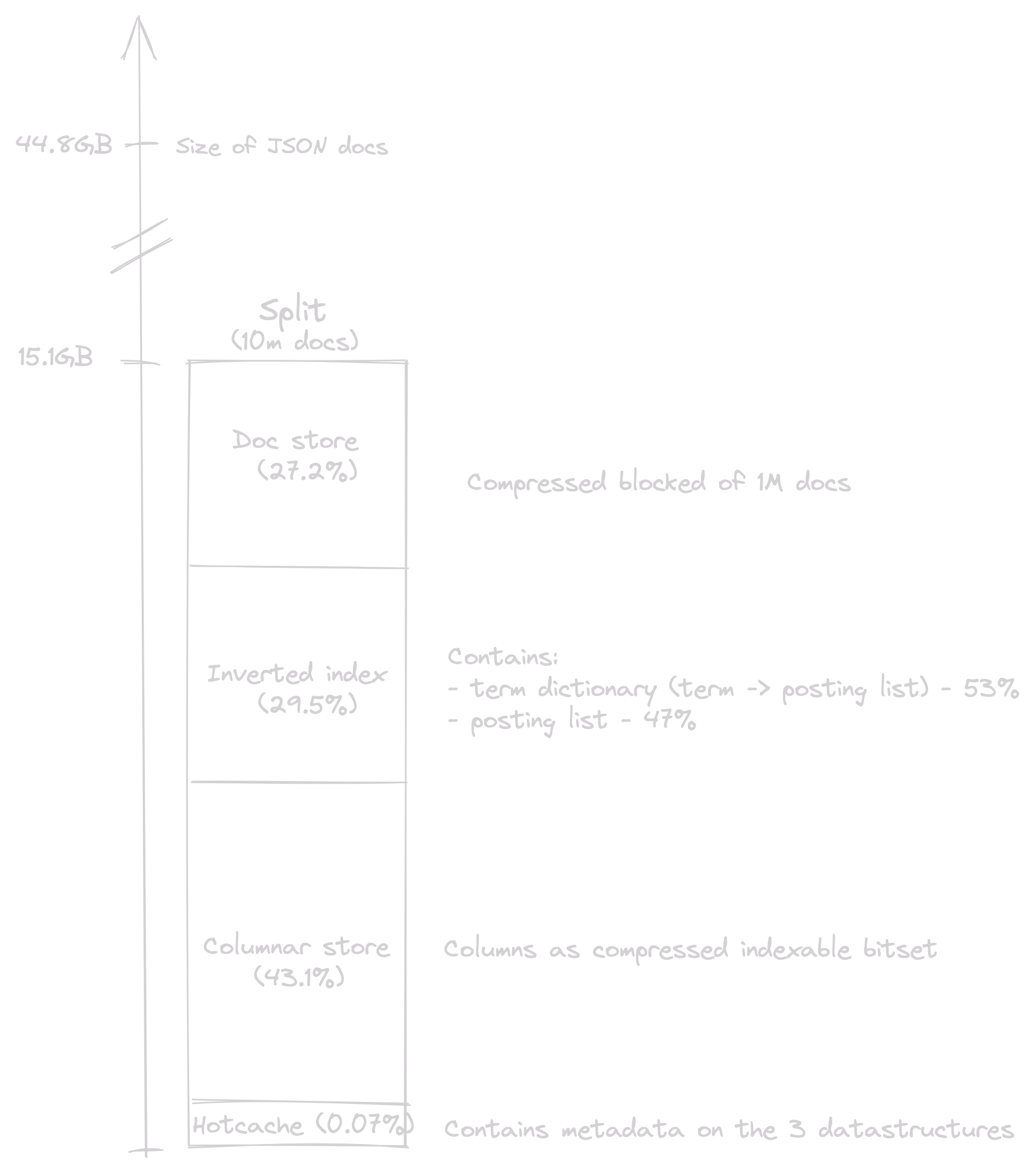
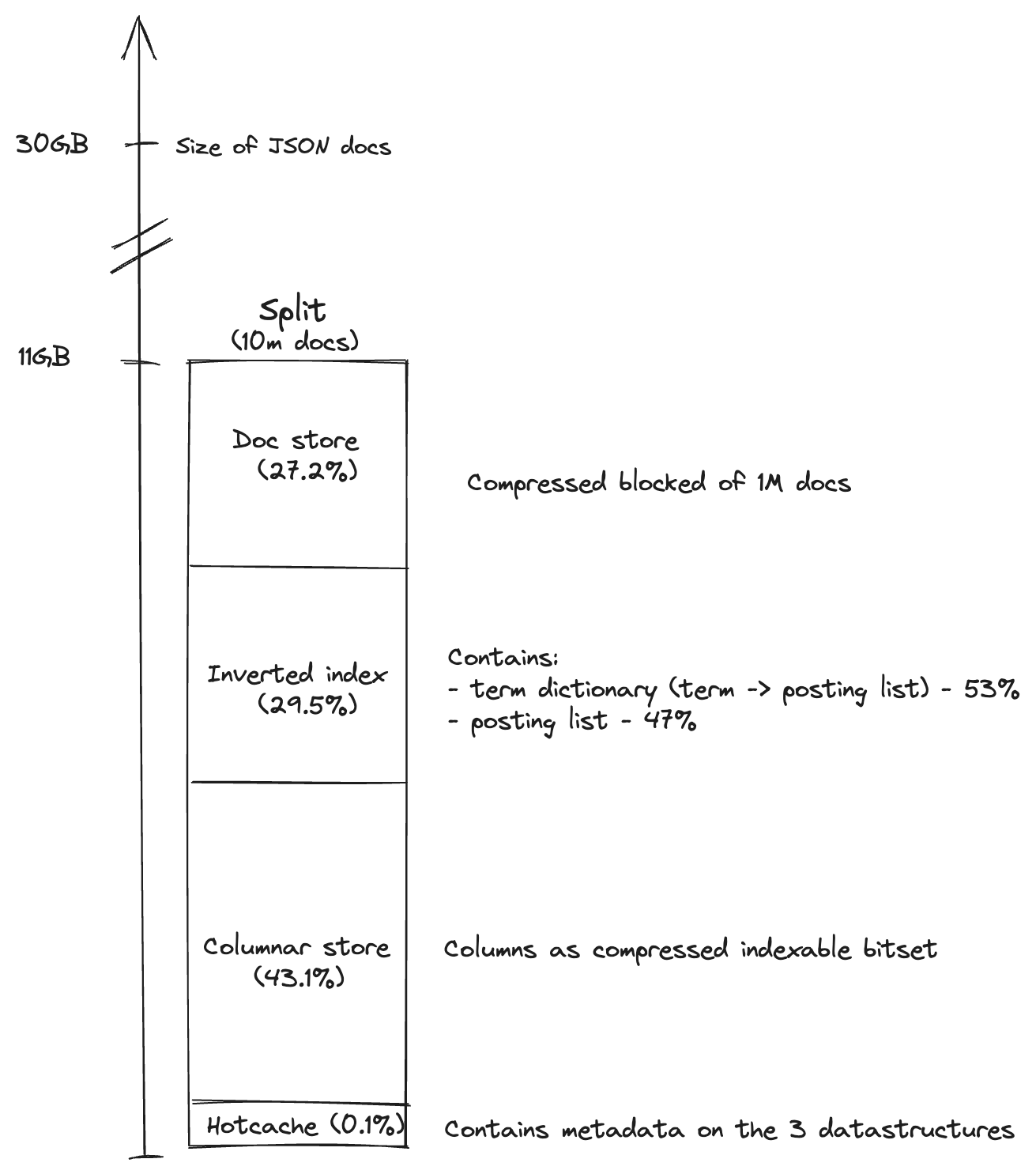
The split size is roughly 15GB. Compared to the uncompressed size of the documents, it shows a compression ratio of almost 3. Note that optimizing this ratio is possible by enabling specific storages only on relevant fields.
Finally, the hotcache shows a nice property: it represents less than 0.1% of the split size, around 10MB, which means it could easily fit in RAM.
A word on merges
You may wonder how Quickwit manages to generate 10 million-document splits while the indexer can commit every 10 seconds. The answer lies in Quickwit's merge pipeline, which takes care of merging a group of splits until it reaches a given number of documents3. This is useful for two main reasons:
- Performance Enhancement: You don't want to open many tiny splits on each search request. It also considerably reduces the amount of data our metastore has to handle. Thanks to merges, we end up having one row in PostgreSQL for every 10 million documents.
- Cost efficiency: You're happy to limit the number of GET requests on each search request.
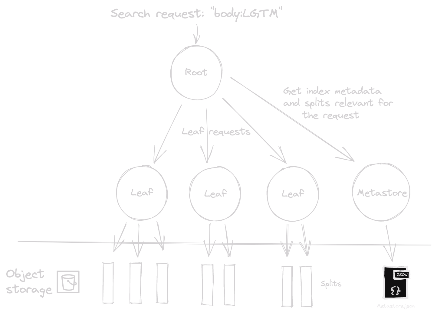
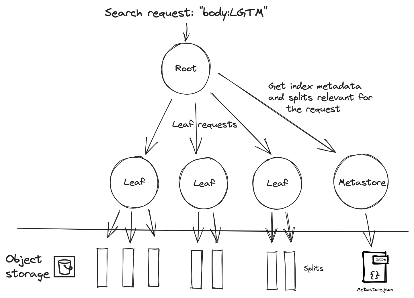
Search
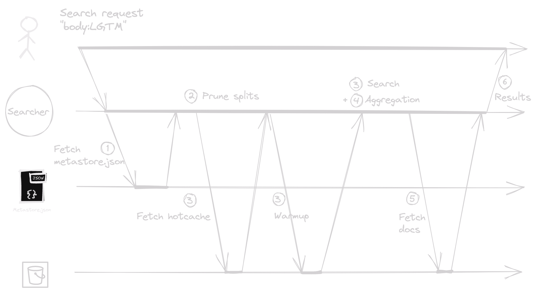
On the read side, when a searcher receives a search request, it goes through these steps:
- Metastore Retrieval: The searcher fetches the
metastore.jsonfile. - Split Listing: It lists relevant splits for the search request. This phase notably uses the search request's time range to eliminate splits that don't match the time range4.
- Leaf Search Execution: For each split, a concurrent « leaf search » is performed. It includes:
- (IO) Retrieving the split's hotcache.
- (IO) Warmup phase: For each term, it fetches the posting list byte ranges and then the posting list itself. If necessary, it also fetches positions and columns required for the search5. For readability, the warmup phase is represented as a single fetch on the diagram below, but in reality, it can be multiple fetches.
- (CPU) Search phase: Runs the query on the split.
- Result Aggregation: The leaf search results are merged.
- Document Fetching: The searcher fetches the documents from related splits.
- Result Return: The matching documents and/or aggregations are finally returned to the user.
This results in the following read path:

The Metastore
Let's return to the shared view of indexers and searchers: the metastore. It stores the critical information about the index that we partly saw in the previous sections:
- Index configuration: document mapping, timestamp field, merge policy etc.
- Splits Metadata: If your dataset has a time field, Quickwit notably stores the min and max timestamp values for every split, enabling time-based filtering at search time.
- Checkpoints: For every datasource, a "source checkpoint" records up to which point documents have been processed. If you use Kafka as a datasource, the checkpoints contain each partition's start and end offsets indexed in Quickwit. That's what unlocks the exactly-once semantics.
The metastore can be powered by PostgreSQL or a single JSON file stored on the object storage. The latter is used for this blog post as it's the most straightforward setup. Here's a snapshot of the metastore's content:
{
    "index_uri": "s3://indexes/{my-index}",
    "index_config": {...},
    "splits": [
        {
            "split_id": "...",
            "num_docs": 10060714,
            "split_state": "Published",
            "time_range": {
                "start": 1691719200,
                "end": 1691936694
            },
            "split_footer": {
              "start": 1612940400,
              "end": 1616529599
            }
            ...
        }
    ],
    "checkpoints": {
      "a": "00000000000000000128",
      "b": "00000000000000060187",
      ...
    }
}
Did you notice the intriguing split_footer field? That's... the byte range of the hotcache!
Distributing Indexing and Searching
Distributing indexing and search introduces some challenges:
- Cluster Formation: Quickwit uses an OSS implementation of Scuttlebutt called Chitchat to form clusters.
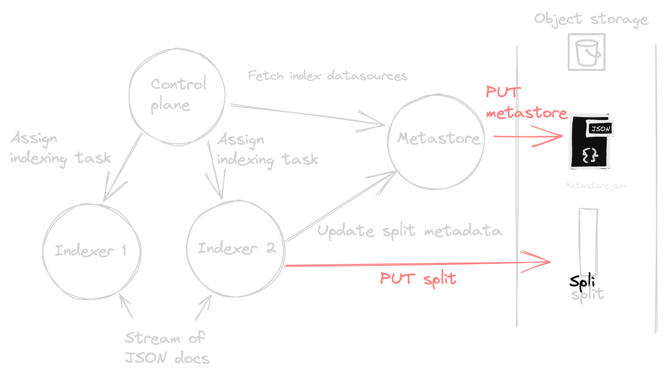
- Metastore Writes: On the write path, only one process should process the writes to the metastore file6. To this end, a single
metastorerole instance reads/writes the JSON file. Other cluster members send read/write gRPC requests to this instance. - Indexing Task Allocation: One control plane role oversees indexing tasks distribution to individual indexers.
- Search Workload Distribution: This requires a map-reduce mechanism. The searcher receiving a search request assumes the "root" role, delegates leaf requests to "leaf nodes", then aggregates and returns the results.
Here's a visual representation of the write path:

Similarly, for the read path:
For a more comprehensive dive, explore our documentation.
Wrapping up
That's it for this first dive, I hope you enjoyed it! For those eyeing performance metrics and costs, we recently published a blog post that benchmarks Quickwit on a 23TB dataset.
Last but not least, there's something on the horizon we're very excited about: our upcoming distributed ingest API. At present, scaling indexing requires users to lean on Kafka or GCP PubSub sources. But with this new feature, you can expect indexing speeds of several GB/s, without depending on external distributed message queues. As we roll this out, we will accompany the next release with a series of blog posts into Quickwit's inner workings. Stay with us!
- This approach is not new in the analytics realm but is more recent in search. Elastic recently published (October 2022) a blog post announcing the evolution of their architecture to a decoupled compute and storage model. You can read more about it here.↩
- PostgreSQL remains the recommended implementation for significant use cases or if you manage many indexes. We will add other implementations in the future.↩
- The default merge policy merges 10 splits until reaching 10 million documents.↩
- The searcher can also prune splits based on query terms using tags. See more details in the docs.↩
- The term's posting list corresponds the list of document IDs containing this term. For a simple term query, it first fetches the byte range of the term posting list, then the posting list itself.↩
- This is not the case with a Postgresql-backed metastore.↩