Search performance on AWS Lambda
This technical blog post is part of a series about Quickwit's serverless performance on AWS S3 and Lambda.
Last week, we announced Quickwit's serverless search on AWS Lambda and S3. Building a sub-second search engine on terabytes of data stored on S3 is challenging. The constrained environment of AWS Lambda makes it even harder. In this post, we dive into Quickwit's search performance on AWS Lambda using a dataset of 20 million log entries.
Benchmark setup
Dataset
Our benchmark uses a dataset of 20 million HDFS log entries. Below is a sample log entry:
{
  "timestamp":1460530013,
  "severity_text":"INFO",
  "body":"PacketResponder: BP-108841162-10.10.34.11-1440074360971:blk_1074072698_331874, type=HAS_DOWNSTREAM_IN_PIPELINE terminating","resource":{"service":"datanode/01"},
  "attributes":{"class":"org.apache.hadoop.hdfs.server.datanode.DataNode"},
  "tenant_id":58
}
The total uncompressed size of the file is 7GB. Once indexed, its size goes down to 1.3GB and it is divided into 8 splits, a split being a small independent piece of the index (Quickwit could be configured to output fewer or more splits).
Queries
We run two types of queries:
- A term query searching for error logs in the dataset. This query uses the inverted index and requires fetching only small data chunks from S3. It is typically not very cpu-intensive.
{"query": "severity_text:ERROR", "max_hits": 10}
- An aggregation query that generates a date histogram for each severity term. This query requires to go through both the timestamp and the severity text fields, which involves more data download and processing than the term query.
{
  "query": "*",
  "max_hits": 0,
  "aggs": { "events": { "date_histogram": { "field": "timestamp", "fixed_interval": "1d" },  "aggs": { "log_level": { "terms": { "size": 10, "field": "severity_text", "order": { "_count": "desc" } } } } } }
}
Lambda configurations
The RAM configuration on AWS Lambda also controls the CPU allocation. We execute our queries on the following configurations (with the approximate associated vCPUs):
| Provisioned Memory (MB) | vCPU Quota |
|---|---|
| 1024 | 0.6 |
| 2048 | 1.2 |
| 4096 | 2.3 |
| 8192 | 4.6 |
The network allocated to the functions is not really specified by the AWS Lambda documentation, but from our experiments, the total bandwidth doesn't really depend on the Lambda configuration and tops at around 80MB/s. Note that for RAM configurations with less than 1 vCPU associated, this bandwidth is often not reachable (our guess is that either the bandwidth is throttled or the CPU is not fast enough to read that much data from the network interface).
Latency control
We observed significant latency variance in AWS S3 queries:
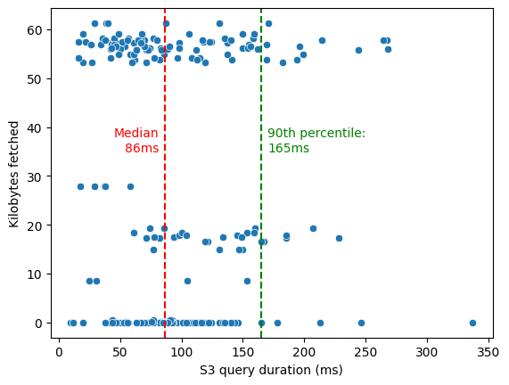
Each dot in this graph represents a download from S3, measured while executing the term query six times on a 1GB Lambda. The download sizes vary, but for term queries, they don't exceed 65KB. Despite the small size, latency can range from 15 milliseconds to a few hundreds. The 90th percentile indicates that 10% of queries exceed 165ms.
To better control the impact of this high variance on our subsequent test queries, we run them at least 10 times for each datapoint.
Caching layers
It is a common belief that we cannot cache data on AWS Lambda. That's not true. Lambda re-uses containers as much as possible across subsequent runs. Two kinds of cache can be leveraged:
- The static context in memory: when invoked, the Lambda runtime executes a configured handler function. However, the static context of the provided binary is only loaded during cold starts and reused across subsequent calls. We can thus control objects that we want to keep in memory across invocations by making them static.
- The local storage: functions can be configured with up to 10GB of ephemeral storage. The cost of this storage is 0.1%1 of the cost of the RAM allocation, so we shouldn't restrain ourselves from using it!
What's very interesting is that you are not billed for the memory or storage that is used during the time the Lambda function is asleep. It's a huge opportunity for both speed improvement and cost saving on subsequent queries:
- Faster execution -> lower Lambda costs
- Fewer calls to the storage -> lower S3 costs
One last thing to mention is the partial request cache (more details about Quickwit cache layers here). This high-level cache gives the second run of the same query an unfair advantage, so we perform our test runs with and without it. Note that use cases where this cache is leveraged are actually pretty common as many applications that use Quickwit as a backend perform some sort of auto-refresh that makes identical queries at regular intervals.
High-level results
We plot the mean billed duration across all runs and a 95% confidence interval.
Let's start with the term query:
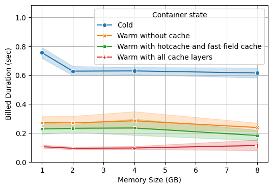
Great news, we consistently get the result within 1 second!
Let's dig a little bit deeper into these results.
The Lambda size has little impact on the query duration, except for the smallest 1GB RAM configuration, which is 30% slower on cold starts. This hints to us that it's the only case where we are CPU-bound.
Second, cold starts are approximately 300ms slower than warm starts. We measured the Lambda initialization time (i.e loading the static context and reaching the Lambda handler) to be approximately 100ms. The remaining 200ms are harder to explain and are most likely related to dependencies that leverage the static context for optimizations.
Finally, we see that only partial caching has a significant impact. The benefit from split footer caching is not noticeable compared with the S3 latency variance.
Let's now take a look at the more challenging histogram aggregation query:
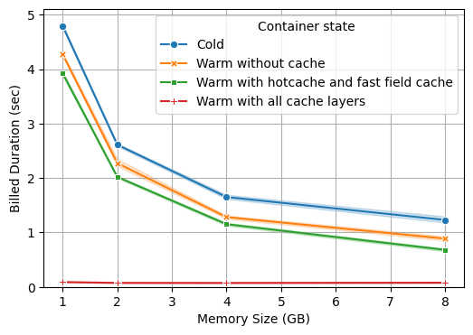
This query is significantly longer than the first one, but with the largest 8GB setup, we are still close to a 1-second duration. Let's unwrap these results.
For the aggregation query, the Lambda size is much more impactful. We are not just leveraging the index for a point search anymore, we need to collect data over the 20 million documents, so this query is much more CPU-intensive than the previous one.
We also get a much clearer benefit from using the cache. On the 8GB RAM Lambda configuration:
- The aggregation takes 700ms on average with the split footer cache and fast field cache, 150ms less than the warm start without cache. Aggregations use the cache more intensively because they store entire fast field columns.
- With the partial request cache the query only checks that the metastore didn't change and serves back the earlier results if it didn't. This cache is very valuable when we plug a client application (such as a dashboard) that has some auto-refresh logic and runs almost identical queries over and over!
Deepdive into the query execution
In the previous section, we discussed high-level results and identified key trends. Now, let's delve deeper by examining individual query executions. We've already noted that S3 downloads often create a bottleneck, so we'll pay special attention to these events.
Term query
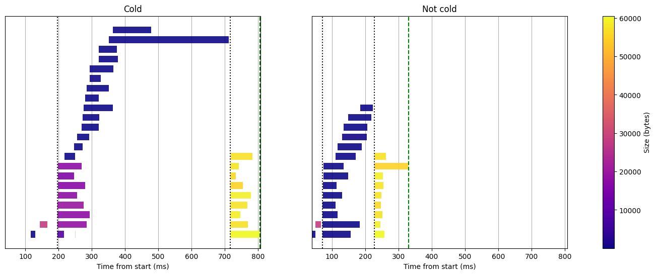
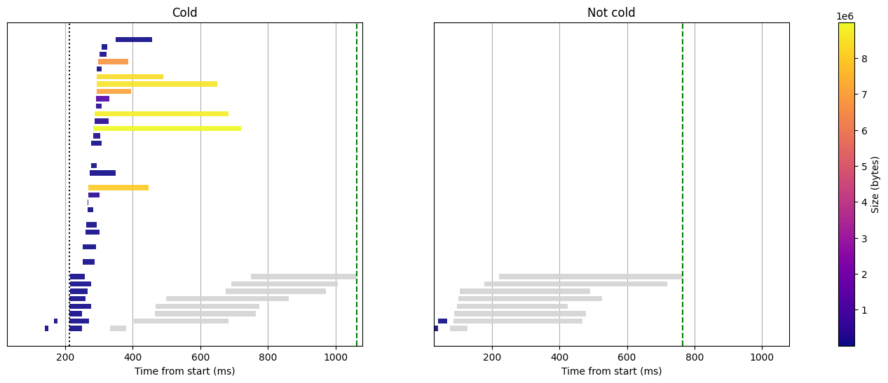
Let's start with the execution of the term query without cache on a Lambda function with 2GB RAM:
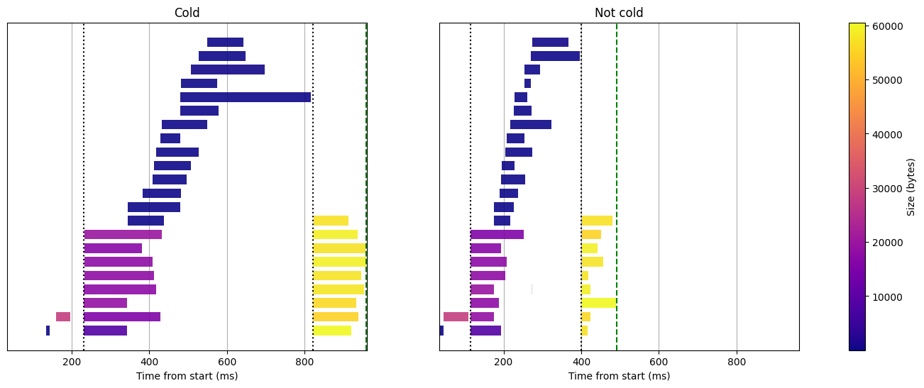
Term query without cache, 2GB RAM
First, let's get acquainted with this visualization:
- The horizontal axis represents the time in milliseconds since the start of the function, not counting the initialization phase.
- Each bar represents a request to S3, its length represents its duration and its color depends on the number of bytes fetched (here between a few bytes and 60KB). This dataset has 8 splits, and we need to download multiple chunks for each of the splits as well as the metastore files.
- The green dashed line represents the end time of the function execution. The
different phases of the query are separated by black dotted lines:
- The first phase is the metastore setup, where we download the two metadata files
(
metastore.jsonandindexes_states.json). - The second phase is the search phase, where we download the various parts of the index that are necessary to find our matches.
- The third and last phase is the docs fetch phase, where we download the actual documents that match our query (this phase is not present for aggregation queries).
- The first phase is the metastore setup, where we download the two metadata files
(
Now let's unpack what's actually happening here. We are not using any cache for now and the Lambda initialization time (i.e execution time before the Lambda handler) is not displayed, so it's interesting to see where the cold start actually spends time.
- First, we see that there is still an extra setup of approximately 150ms at the beginning before the index state is fetched. This is probably related to dependencies that perform some initializations that they cache in the static context.
- Then we observe that queries to S3 are usually much shorter during the second run. The most likely explanation is that some caches get warmed up, such as the local DNS cache or caches within S3.
In this term query, all requests to S3 require only very small chunks of data (up to 65KB). The duration of the query in that case depends only on the latency of S3 and not its bandwidth limitations.
It is also interesting to note that there are some critical paths where a single request to S3 will slow down the entire function. This is the case of the download of the metastore file at the beginning of the function. It also happens with the last fetch from the index, without which the doc scores cannot be sorted and thus fetched.
Interestingly, certain critical paths can slow down the entire function due to a single S3 request. This occurs when downloading the metastore file at the function's start. It also happens during the final index fetch, which is necessary for sorting the document scores and move on to the docs fetch phase.
Let's now take a look at a run of the same query on the same Lambda configuration (2GB RAM), but with the cache enabled:
Term query with hotcache and fastfield cache, 2GB RAM
Before even looking at the effect of the cache on the warm start, we can compare this cold run with the previous one. Most queries to S3 had actually a much lower latency, except one that lasted for more than 300ms and delayed the entire execution. If we hadn't had such bad luck on that single download, the query could have been 100 or even 200ms faster!
Now, let's compare the cold start with the warm start, which utilizes the cache. We observe fewer S3 requests (8 less, to be precise). This reduction corresponds to skipping the download of the split footer for each of the 8 splits. While this does save some time on the critical path, the gain isn't consistently noticeable due to the significant variance in S3 request times.
Let's enable the partial request cache, just for fun. We disabled it when we generated the main results because it's sort of an unfair advantage when running the exact same query a second time. But it's interesting to see what happens to the query phases when it is enabled:
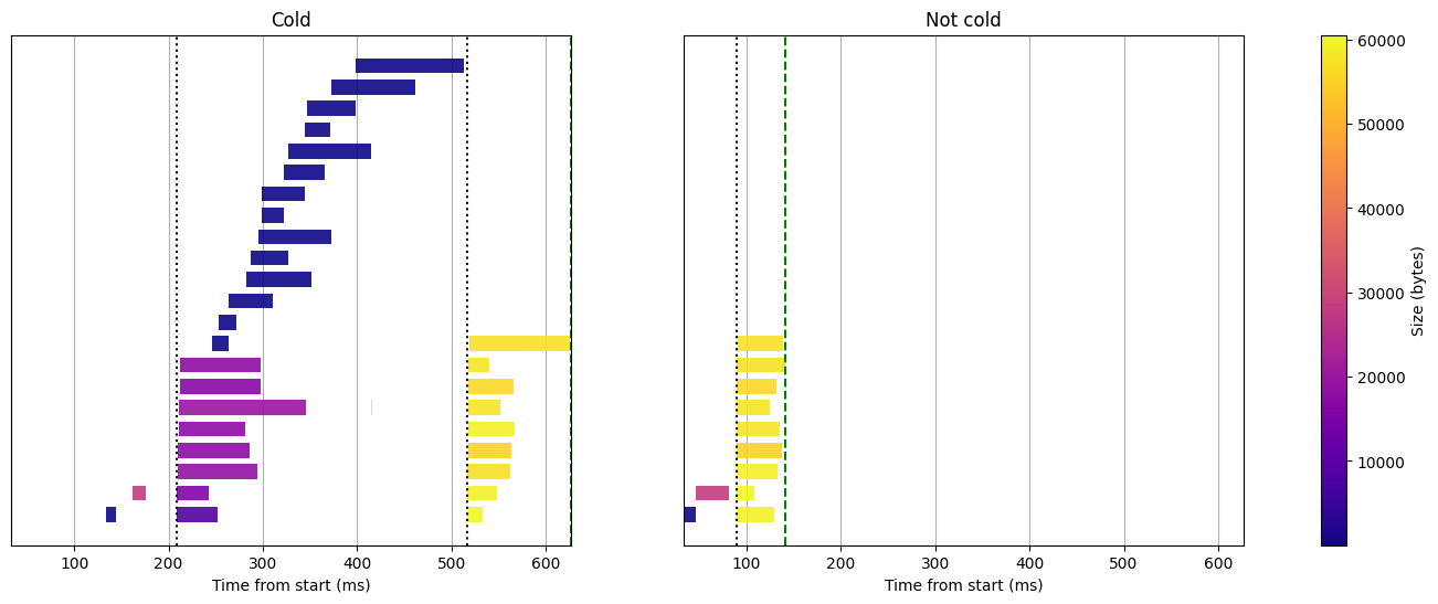
Term query with all caches enabled, including partial request cache, 2GB RAM
Nice, all queries to the indices are skipped! We are left with the download of the metastore files (to check that the dataset didn't change) and the fetch of the docs which aren't cached.
Histogram aggregation queries
Now that we have seen the internals of the term query, let's move on to the histogram aggregation.
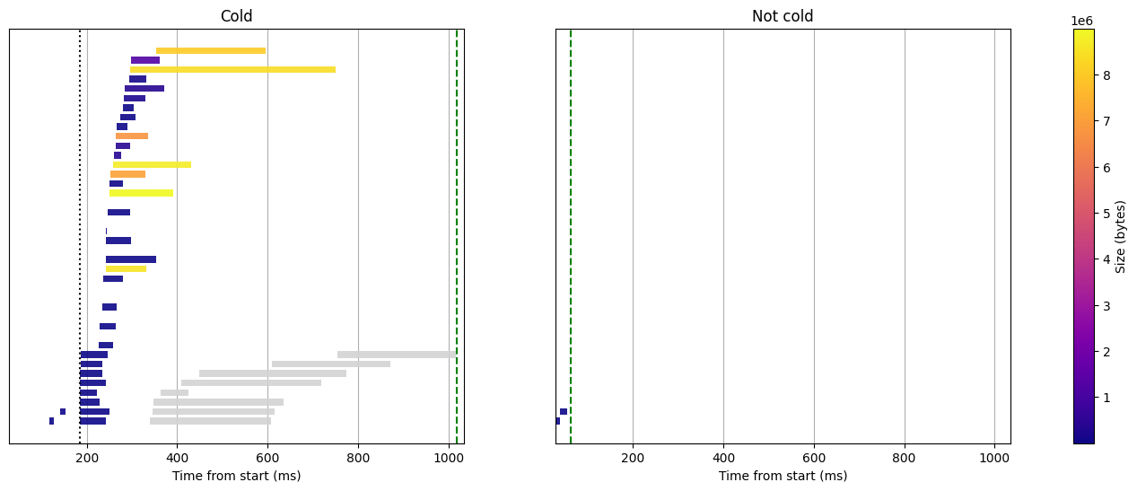
To start, we run the histogram query with the same 2GB RAM Lambda function as the term queries above, and without the cache:
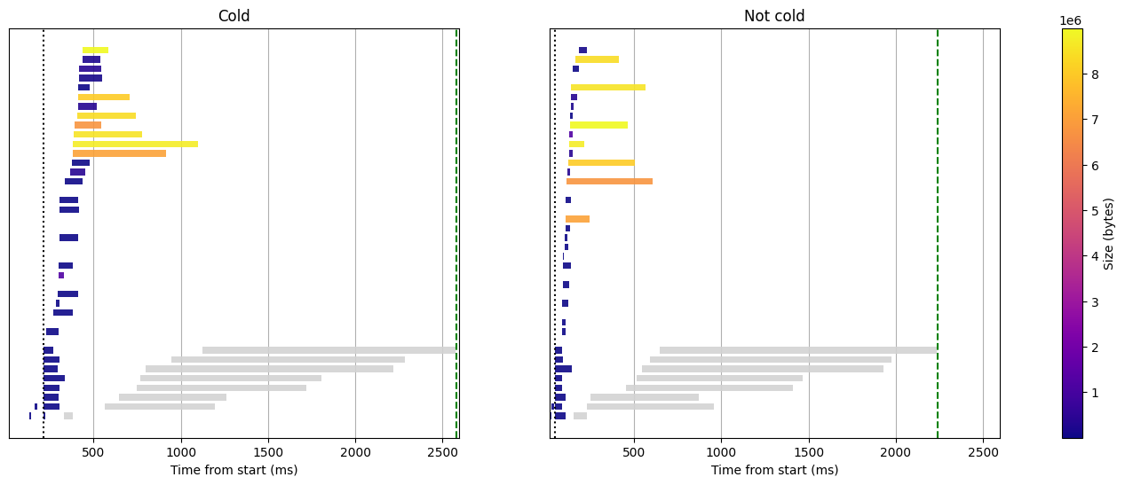
Histogram query without cache, 2GB RAM
The setup of the metastore is the same as for the term query, so there isn't much to say on that first phase.
If you take a careful look at the color scale of the download sizes, you'll notice that the largest size is now around 9MB, that's 150 times the largest download of the term query. Aggregations require downloading entire fast fields (value columns), and even though those are quite optimally encoded by tantivy (the search library used by Quickwit), they remain fairly large. These requests to S3 are fundamentally longer as they hit the bandwidth limitation and no longer solely depend on the request latency.
Now, let's address the elephant in the room. We can notice right away that there is no document fetching phase. Indeed, aggregations are performed on the indexes and we don't gather any documents. But what are these grey bars that popped up? These represent the tantivy processing. They are not part of the color scale because they don't involve any interaction with S3, it's just pure CPU processing. They now take up most of the processing duration. Even though it might look like they are running all in parallel, they don't, they are just concurrent. Remember, we are running on a 2GB function here, and that implies that we have only 1.2vCPU available.
Lets bump the Lambda configuration to 8GB RAM, that should give us approximately 4.6 vCPU:
Histogram query without cache, 8GB RAM
Great, the tantivy processing duration decreased quite drastically! This brought us a little under the 1 second bar for the warm start.
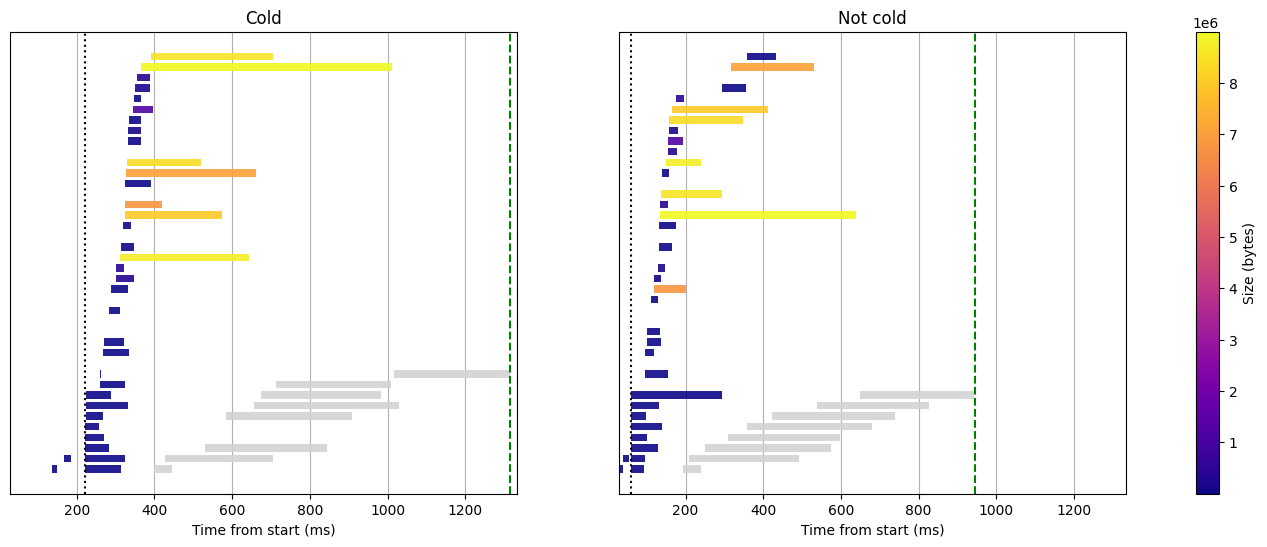
Let's enable the cache to see if we can do better:
Histogram query with hotcache and fastfield cache, 8GB RAM
We are mostly interested in the warm start. The only requests to S3 we still have are those for the metastore. The rest is tantivy at work. That's because both the hotcache (split footer) and the fast fields (value columns) are cached.
If you compare carefully the gray bars between the cold and the warm start, you might get the impression that those of the warm start are longer. It's true. But if you try to measure the time elapsed between the first tantivy processing starts and the last ends, the gap is actually quite anecdotal. In the case of the cold start, the tantivy processing is scheduled progressively as the results come back from S3. Even though the last chunk of fast field comes back more than 700ms after the function started, the utilization of the 4 vCPUs is almost optimal 200ms earlier. And as the concurrency is rarely more than 4, each chunk gets processed faster as they have more CPU resource available. Altogether, we can say that the resource usage is very good:
- When possible, we use the cache provided by Lambda, which is free because we don't pay the used RAM between function invocations
- When the data isn't cached, there is a large portion of the execution where Quickwit is using both the network and the CPU to their maximum.
Now, just for fun, let's do one last execution where we enable the partial request cache:
Histogram query with all caches enabled, including the partial request cache, 8GB RAM
Apart from the metastore fetch, no download, no tantivy processing. The results are just fetched in less than 100ms. Thanks to this cache you might set up an auto refreshing application backed by Quickwit serverless without worrying costs!
Possible improvements
We have identified a few optimizations that we could leverage to further improve serverless search on Quickwit:
- Skip the call to the index state file when we have a unique index per Lambda function. This would spare us the latency of a full round trip to S3 as that call is on the critical path of the function execution.
- We could use a backend with a lower latency for the metastore. For instance we could store it on S3 Express One Zone. We might also consider using DynamoDB.
- The S3 performance guidelines advises to retry slow requests to mitigate the request latency. Configured properly this could decrease the performance variations.
If you are interested in any of these features or other ones, join us on Discord and share your use cases with us!
Appendix: Metric extraction
A cloud function is a constrained environment where all resources are relatively scarce. It is hard to guarantee that the fact of extracting observability data does not impact the execution itself. Here are the most common ways of extracting observability data from AWS Lambda:
- Returning the measurement data points in the function response. But the payload is pretty constrained in size and goes through multiple layers of proxy (Runtime API, Lambda service API...) which might slow down the total execution duration.
- Sending the measurements to an external service. We can make API calls to send out the observability metrics to a self-hosted or managed service. But those calls would need to be monitored themselves to ensure that they don't introduce extra latency. That adds quite a bit of complexity.
- Using the native Cloudwatch Logs setup as a sidepath for observability data. The Lambda instance takes care of collecting textual logs and forwarding them to the Cloudwatch service which makes them queryable.
We decided to use Cloudwatch Logs with structured logging to extract all the KPIs that are displayed in this blog post. The Rust tracing library is highly modular and offers a customizable output for all logging points already configured in Quickwit and its dependencies. This implies a bit more post-processing work, but gives us better confidence that the instrumentation has as little impact on the execution as possible.
- From the AWS Lambda pricing page, $0.000016 for every GB-second of RAM and $0.00000003 for every GB-second of storage.↩